Excel Excel help - vlookup?

Joined
Oct 9, 2012
Messages
10
Reaction score
0
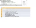
So hopefully I will explain this right and I have attached a print screen also
Sheet one has columns A, B, C
Sheet two has C and D

I want to match these two by the first few letters in B (from sheet 1) and D (from sheet 2)

And to display the results in sheet 2 so that I can also see C

Some of them may not match. Whatever I am doing my formula is not working. Any help from anyone would be VERY much appreciated.
 

Attachments

  • match descriptions.webp
    match descriptions.webp
    29.3 KB · Views: 247
A VLOOKUP formula will look for all of the Lookup Value and look for an EXACT match (or approximate, if you use True as the last arguement, but that only works if things are set up a certain way) for the value in the first column of the lookup array. Below I'll explain the VLOOKUP a little more specifically, but first I just wanted to inquire to see if you are looking to match only the first 3 characters from one to the other, or exactly how you're doing the lookup.

A VLOOKUP is as follows:
1st Argument: Lookup Value, the value you are matching to the first column in a table
2nd Argument: Table Array, the table that has the first column of IDs that you want to match the Lookup Value to, and also contains the data that you want to extract, to the right of the column containing the match for the lookup value
3rd Argument: Column Index Number, this is the number of the column within the table array that you want to pull the data from when the value on that row matches the lookup value
4th Argument: Range Lookup, You will use False here to look for an exact match for your Lookup Value in the first column of the table array. You will use True here to look for an approximate match for your Lookup Value in the table array. For this to work, the data in the Table Array needs to be sorted in Ascending Order on the first column.

With the explanation here, I don't think that the VLOOKUP will do what you need without either adding a working column of IDs that will make things match for and rearranging your data. However, if you can explain a little more fully (how many characters you want to match on, what happens if there is no match, etc) I might be able to come up with something that will work for you.
 
thanks for the reply.
i just want to get it to match as much as possible, for the ones that dont match I will do it manually. if it could match the first few characters, maybe 4, then it should do a pretty good job....if i can get it to work :-)
can you give any suggestions?
 
alow describes the vLookup function correctly. As stated, there are a couple of things to remember when deploying a formula to seek results. First, the formula will not distinguish the text. You will need to have absolutes in the values in order to use a formula to glean the results. Additionally, the vLookup formula only returns the first result in the series. If you have multiple matches you will not be able to capture them with vLookup.

I did not see anything even close to a match in your screenshot. If you are able to show some correlation between the records it may be possible to add some commands to the formula such as Right, Trim, Mid, and other string functions. You might even be able to deploy text-to-columns if you have mixed strings with common delimiters.

Steve
 
I could be barking up the wrong tree altogether but:

(See attached)
The description will be the same in both sheets, but one sheet has a system code and description.
The other sheet has an internal code an a description.

I want to get on one line, by matching them up (description is the common field),
Internal code, description, system code.

Does this make more sense??
 
To try this out, assuming you have at least some exact matches in the description, is first in Sheet two, switch the data in columns C and D so you have the description in Column C and the number in Colum D. Then go to column D in sheet one and try something like the following formula:

=VLOOKUP(B2,Sheet2!$C$1:$D$100,2,0)

This is assuming that you are starting in the 2nd row on sheet 1 and that your data in sheet 2 goes down 100 rows. You can change the row number accordingly. You also may need to change the sheet name for sheet 2 in the expression. If sheet 2 has a name with any spaces in it, you will need to change it in the formula as follows: 'Name of Sheet 2'!.

Let me know how that works for you!
 
I'll take it to mean that it worked for you! Glad you got it sorted out :thumb:
 
can i ask one more question that you may or may not know.
does the description in row 1 have to match the description in row two for this to work??
for example if the descriptions were all over the place like monday was on row 5 in one sheet and monday was on row 10 in sheet two, could they be matched this way??
 

Attachments

  • example.webp
    example.webp
    33.8 KB · Views: 371
It will work, regardless of location with the following criteria being met:
  • You have 0 or FALSE as the last argument of the VLOOKUP
  • There is an EXACT match to be found in the table array
  • There is only ONE EXACT match to be found in the table array
If all those are met, then you don't have to have the tables sorted or in a certain position to get the results you need, but you do need exact matches.
 
Back
Top